NEON

Canopy Height from Space

The National Ecological Observatory Network has invested in high-resolution airborne imaging of their field sites. Elevation models generated from LiDAR can be used to map the topography and vegetation structure at the sites.

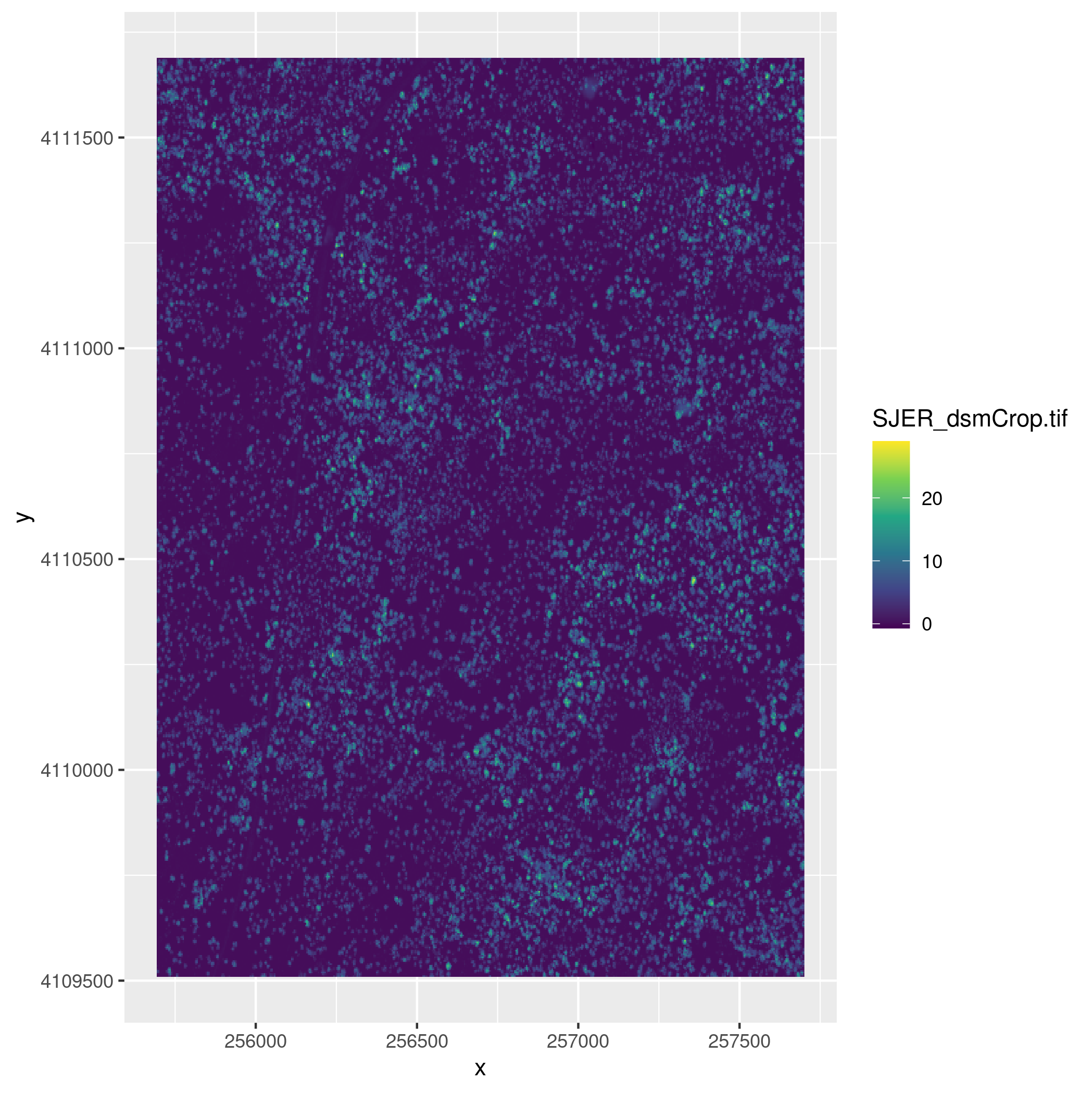
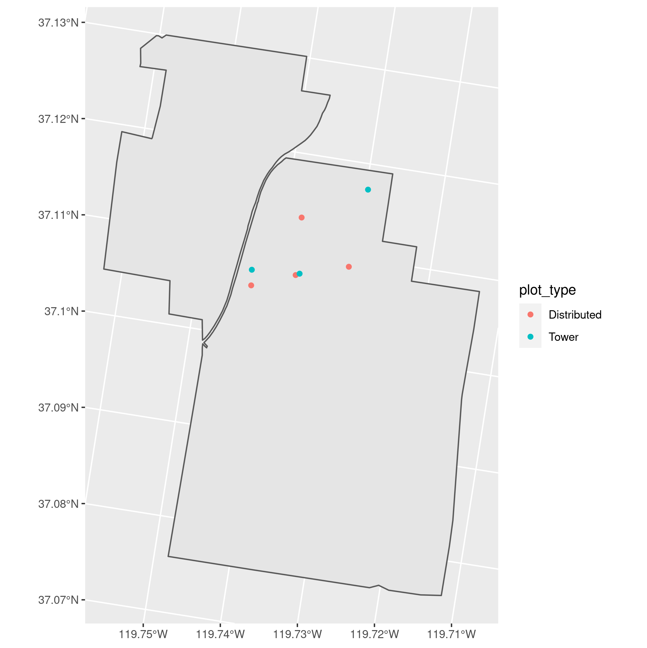
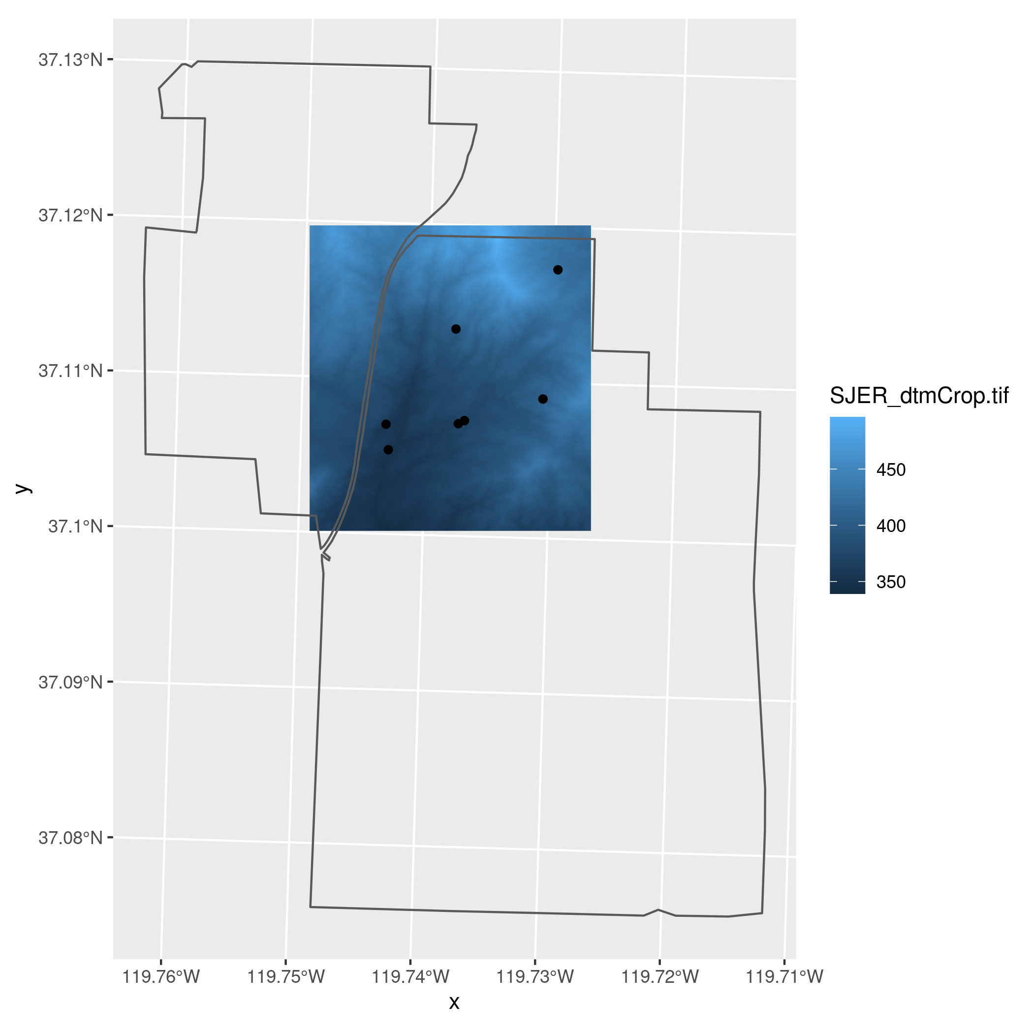
Check to see if there is a data directory in your workspace with an SJER subdirectory in it. If not, Download the data and extract it into your working directory. The SJER directory contains raster data for a digital terrain model (sjer_dtmcrop.tif) and a digital surface model (sjer_dsmcrop.tif), and vector data on plot locations (sjer_plots.shp) and the site boundary (sjer_boundar.shp) for the San Joaquin Experimental Range.

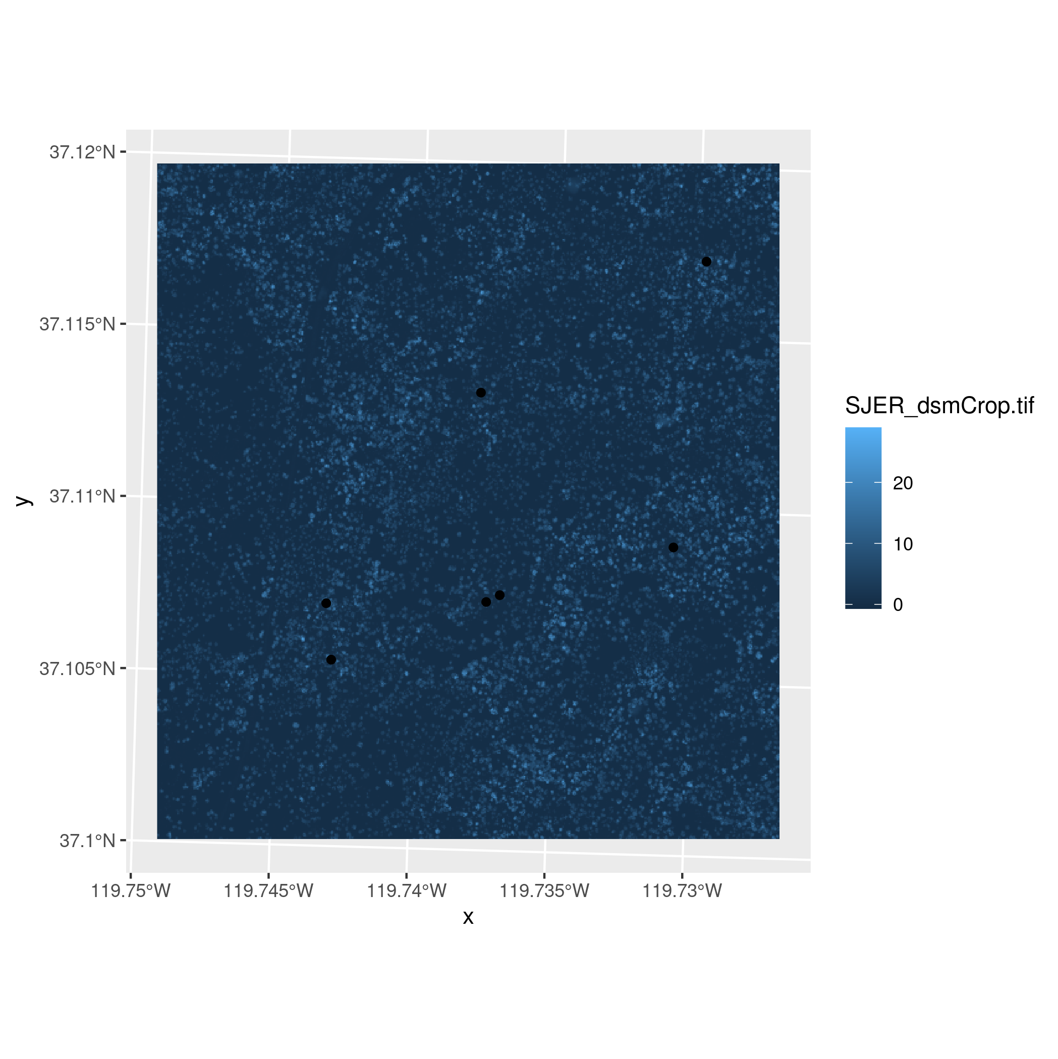
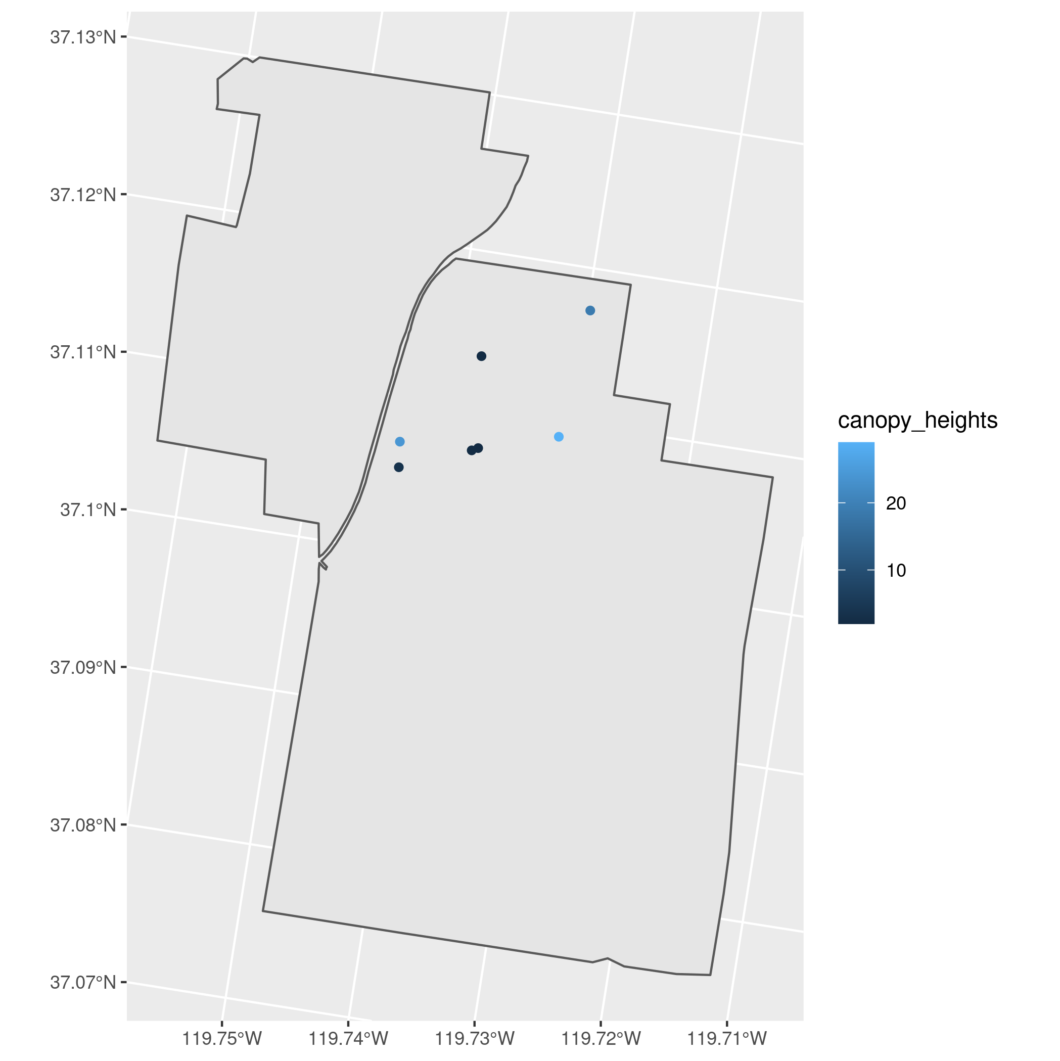
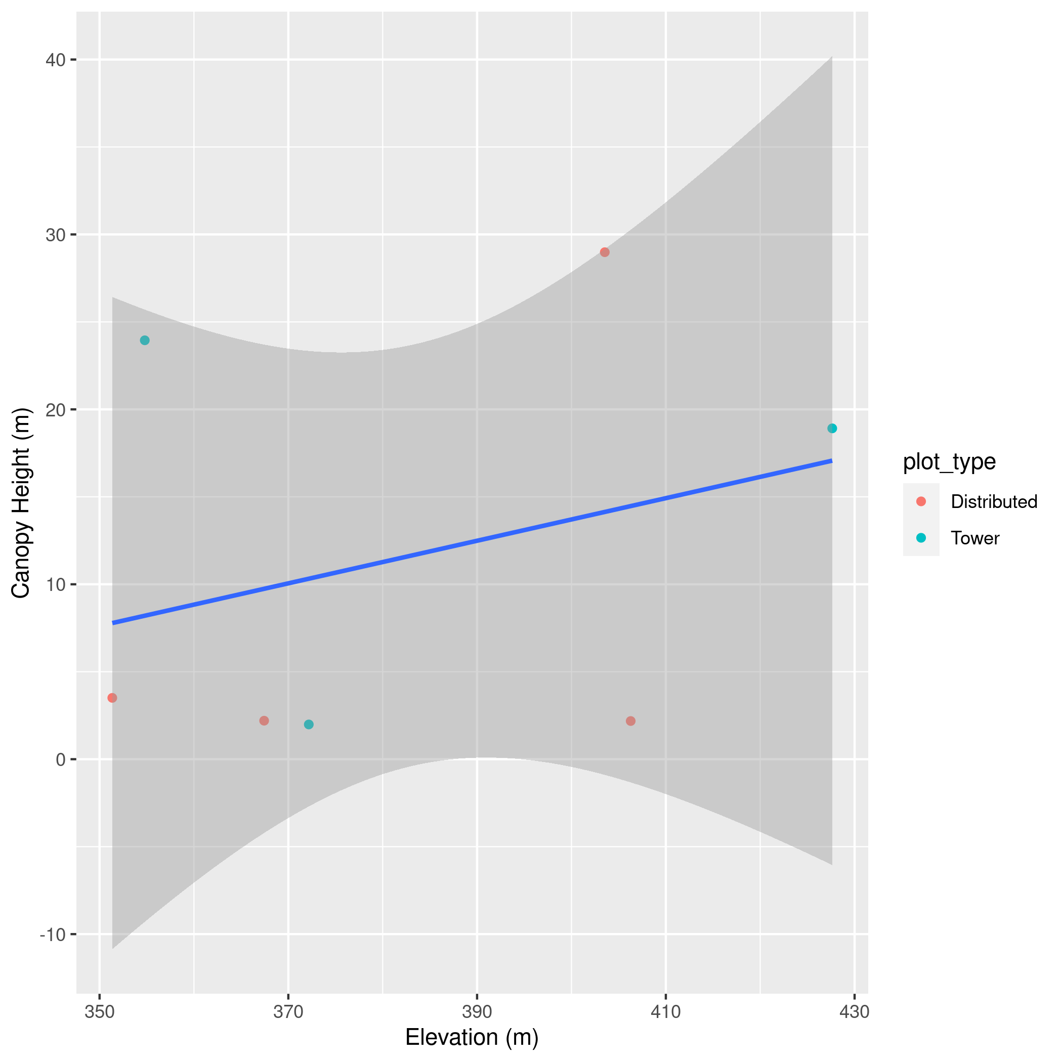
1. Map the digital terrain model for SJER using the viridis color ramp.
2. Create and map the canopy height model for SJER using the viridis color ramp. To do this subtract the values in the digital terrain model from the values in the digital surface model using raster math (chm = dsm - dtm).
3. Create a map that shows the SJER boundary and the plot locations colored by plot_type.
4. Transform the plot data to have the same CRS as the CHM and create a map that shows the canopy height model from (3) with the plot locations on top.
5. Extract the mean canopy heights at each plot location for SJER and display the values.
6. Add the canopy height values from (5) to the spatial data frame you created for the plots and display the full data frame.
7. Create a map that shows the SJER boundary and the plot locations colored by the canopy height values.
8. Create a map that shows the canopy height model raster, but in cm rather than m (i.e., multiply the canopy height model by 100).
9. Create a map that shows the digital terrain model raster, the plot locations, and the SJER boundary, using transparency as needed to allow all three layers to be seen. Remember all three layers will need to have the same CRS.
10. (optional) Conduct an analysis of the relationship between elevation and canopy height at the SJER plots. Start by extracting the mean elevations (i.e., the values from the digital terrain model) at each plot location for SJER and adding them to the spatial plots data so that this data now includes both the elevations and the canopy heights. Then make a scatter plot showing the relationship between elevation and canopy height using this data. Color the points by plot_type and fit a linear model through all of the points together (not separately by plot_type). Finally, use dplyr to calculate the average canopy height and average elevation for the two different plot types. Give the axes good labels.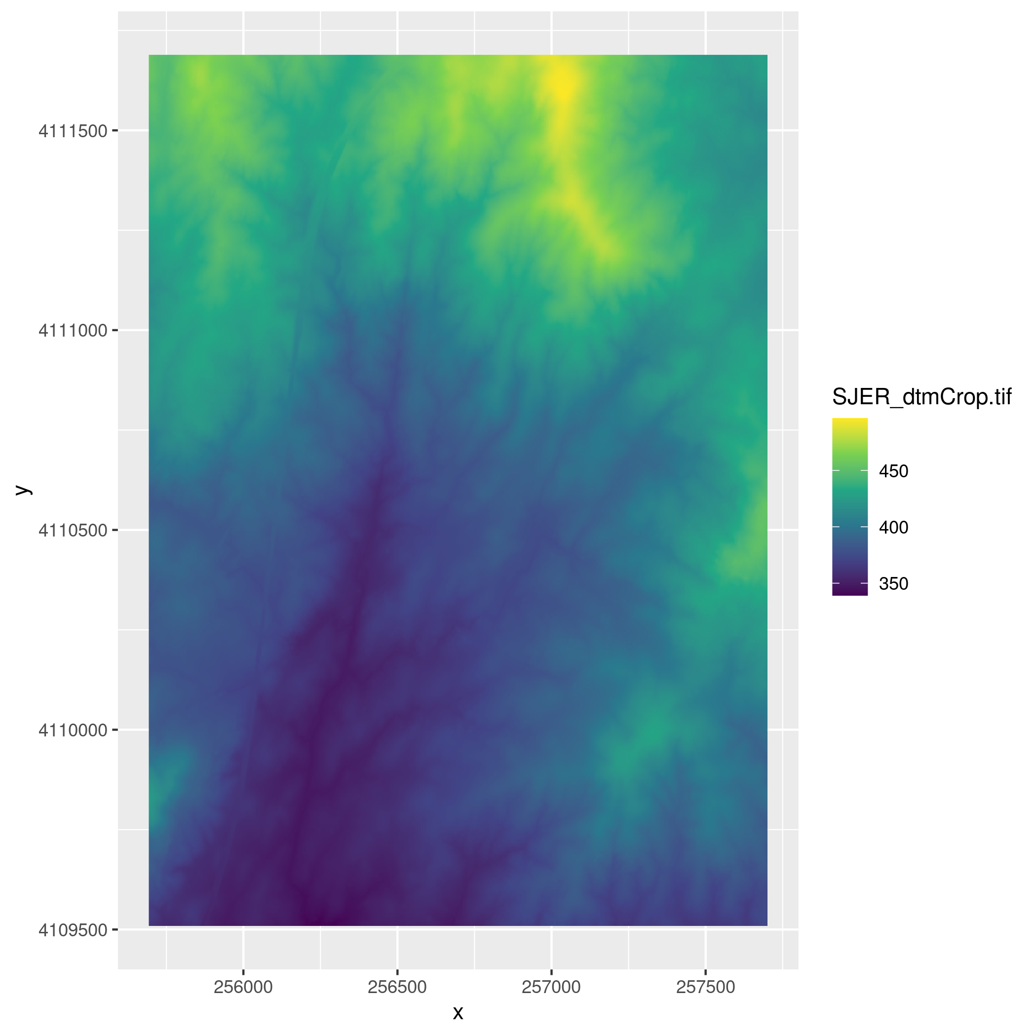

[click here for output] [click here for output] [click here for output] [click here for output] [click here for output] [click here for output] [click here for output] [click here for output] [click here for output]