Graphing

Acacia and Ants Histograms

An experiment in Kenya has been exploring the influence of large herbivores on plants.

Check to see if ACACIA_DREPANOLOBIUM_SURVEY.txt is in your workspace. If not, download it. Read it into R using the following command:

acacia <- read.csv("data/ACACIA_DREPANOLOBIUM_SURVEY.txt", sep="\t", na.strings = c("dead"))

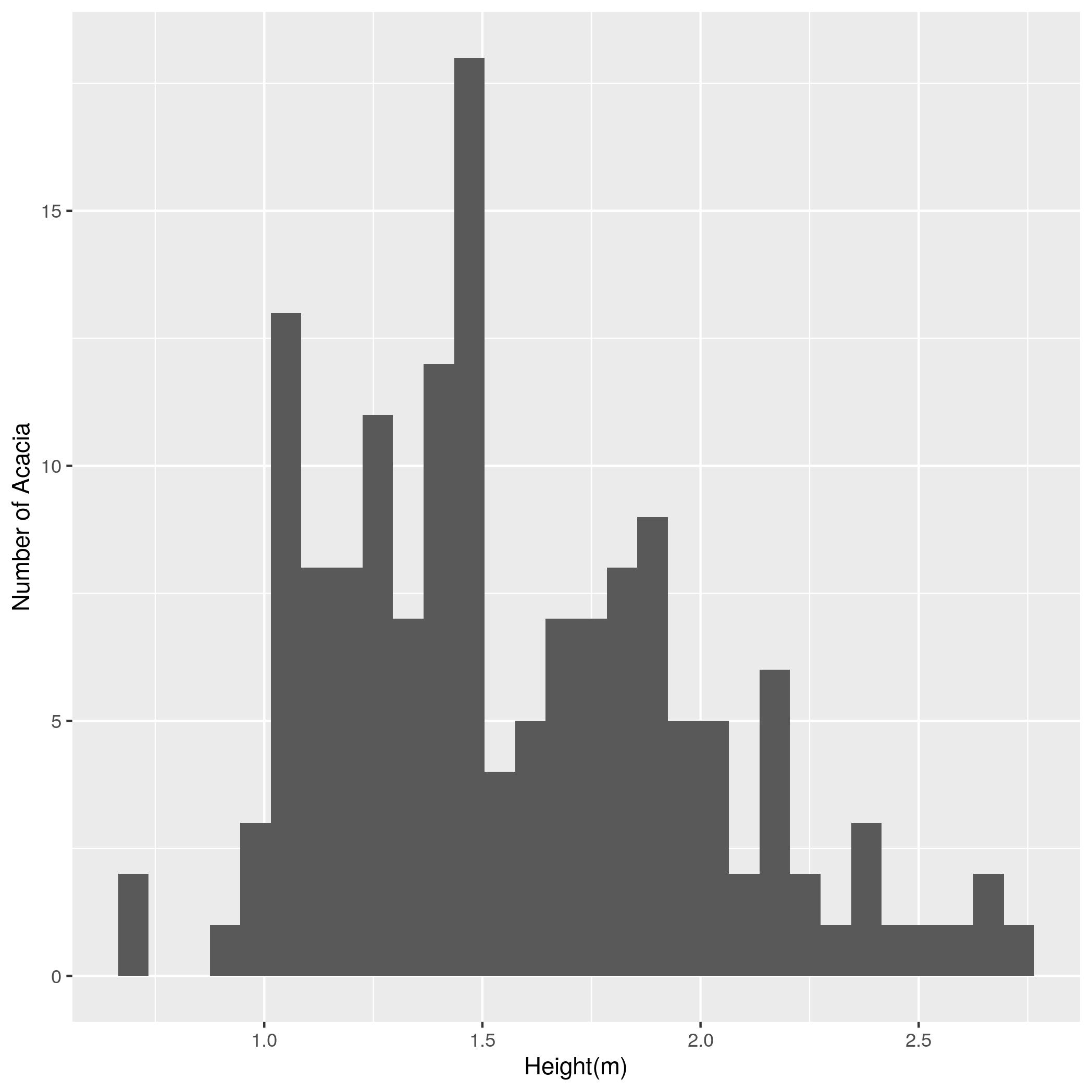
Make a bar plot of the number of acacia with each mutualist ant species (using the ANT column).
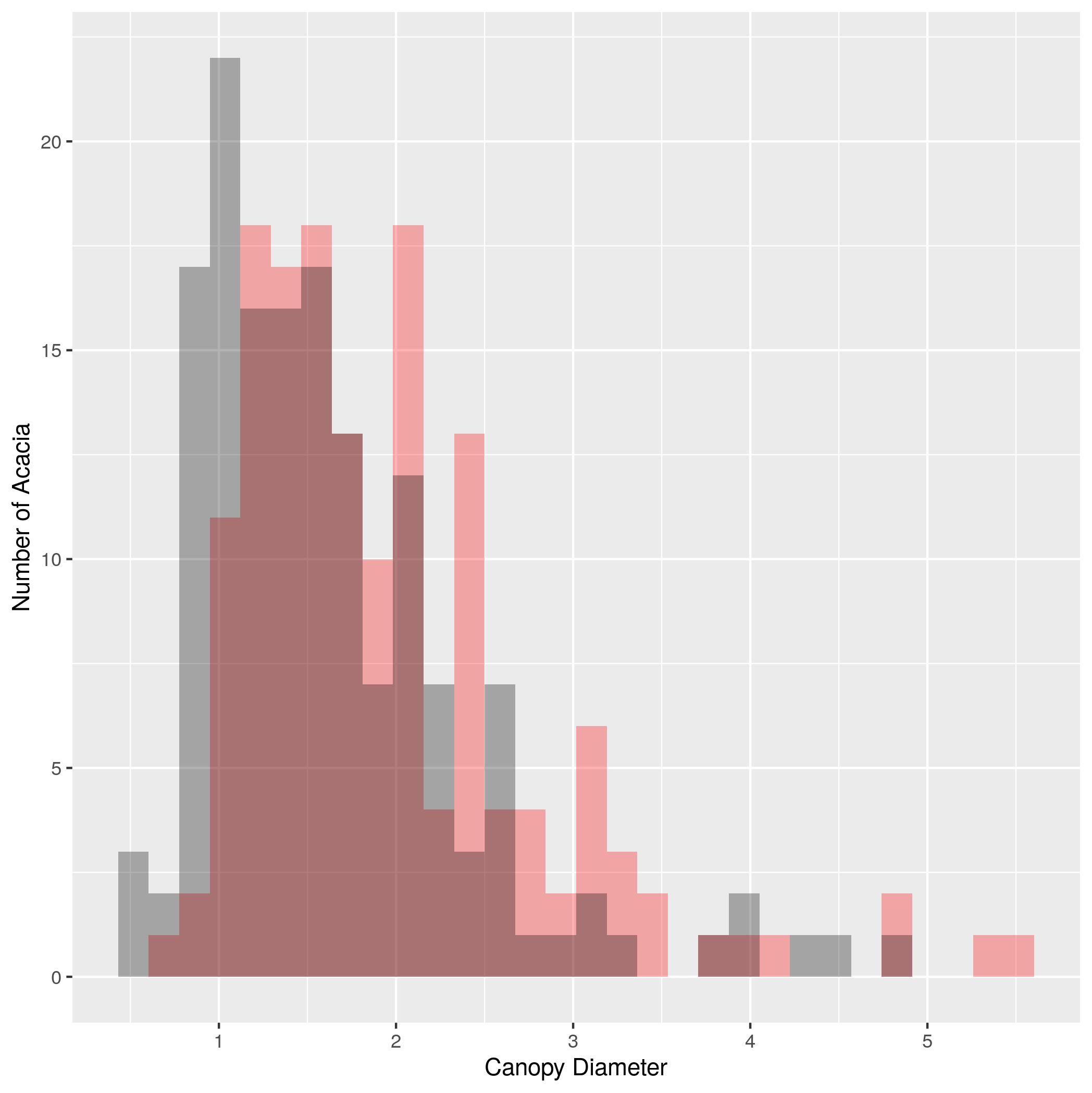
Make a histogram of the height of acacia (using the HEIGHT column). Label the x axis “Height (m)” and the y axis “Number of Acacia”.
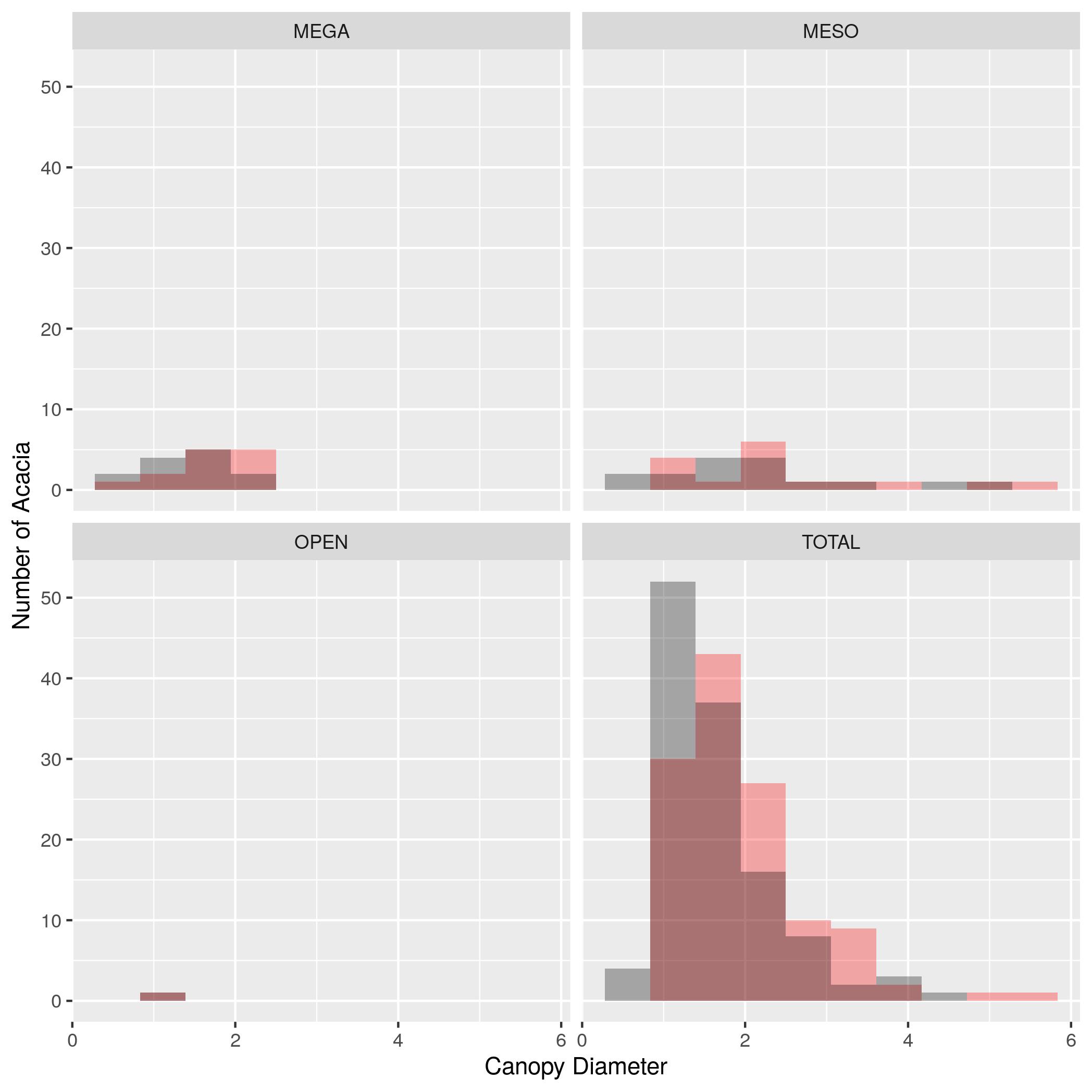
Make a plot that shows histograms of both AXIS1 and AXIS2. Due to the way the data is structured you’ll need to add a 2nd geom_histogram() layer that specifies a new aesthetic. To make it possible to see both sets of bars you’ll need to make them transparent with the optional argument alpha = 0.3. Set the color for AXIS1 to “red” and AXIS2 to “black” using the fill argument. Label the x axis “Canopy Diameter(m)” and the y axis “Number of Acacia”.
Use facet_wrap() to make the same plot as (3) but with one subplot for each treatment. Set the number of bins in the histogram to 10.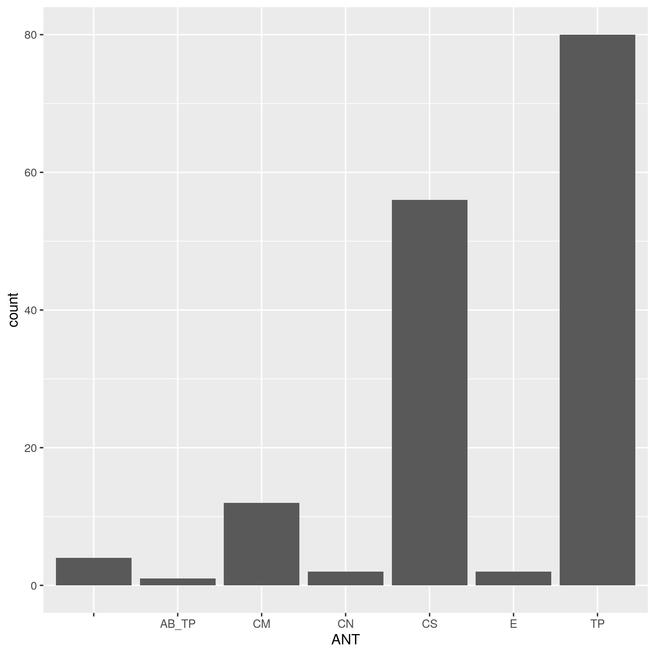

[click here for output] [click here for output] [click here for output] [click here for output]